There are many different ways to interpret the linear regression framework. Below I document the ones I have found useful.
The general problem is that we want to predict some variable Y based on some inputs X1 up to Xp. If we assume this relationship is linear then we would have \(Y = \beta_0 + \beta_1 X_1 + \cdots + \beta_p X_p\)
Note here we are assuming that the real world relationship between the X and Y variables is as above. Then, based on our samples we try to estimate what the beta is.
Simple minimising sum squares
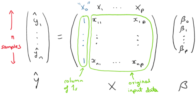
Suppose we have \( n \) samples of data. We define:
- \( Y \in \mathbb{R}^n \): vector of observed outcomes
- \( X \in \mathbb{R}^{n \times (p+1)} \): matrix with the first column consisting of 1s (for the intercept), and each subsequent column corresponding to one input variable
- \( \beta \in \mathbb{R}^{p+1} \): vector of parameters
Then the predicted values are given by $$\hat{Y} = X \beta $$
We want to choose \( \beta \) to minimise the sum of squared residuals: $$\text{RSS} = (\hat{Y} – Y)^\top (\hat{Y} – Y) = (X \beta – Y)^\top (X \beta – Y)$$
To find the minimiser, take the gradient of RSS with respect to \( \beta \) (see this post on matrix calculus): $$\nabla_\beta \text{RSS} = 2 X^\top (X \beta – Y) $$
Setting this gradient to zero gives: $$ X^\top X \beta = X^\top Y$$
Assuming \( X^\top X \) is invertible, the solution is: $$ \hat{\beta} = (X^\top X)^{-1} X^\top Y $$
Geometric view
The expression \( X \beta \) is just a linear combination of the columns of X, with coefficients beting the \( \beta s\).
Hence the problem reduces to finding the unique point in span(columns of X) which is closest to our observed values of Y. Here “closest” is in terms of euclidean distance (which one can easily see reduces to the same residual sum of squares).
We illustrate this in the picture below where the span(columns of X) is shown as a plane. Note this includes the columns of 1s.
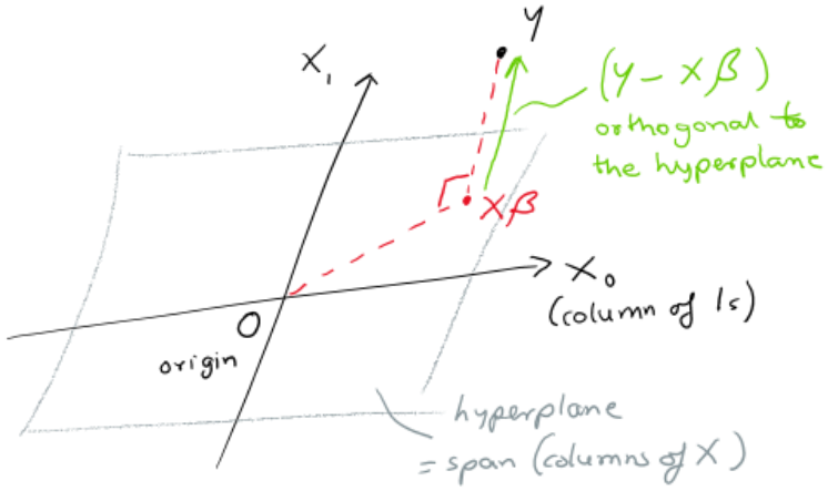
Then we want the point \( X \beta \) that is closest to Y. This is equivalent to saying that the vector \( Y – X \beta \) is orthogonal to the plane (ie orthogonal to each column of X). This means we want the dot product
\(
\left( (Y – X \beta) \cdot i^{th} \,column\, of \, X \right)= 0
\) for all i. This can just be written as
\( X^\top \cdot (Y – X \beta) = 0 \) which gives
\( \hat{\beta} = (X^\top X)^{-1} X^\top Y \)
Standard error in the Beta estimate
So far, we’ve treated estimating \(\beta\) as a purely numerical task: given \(n\) samples, find the \(\beta\) that minimises the sum of squared errors. But to calculate confidence intervals, we need a richer model. We now assume that the real world relationship between the variables is: $$Y = X\beta + \epsilon$$
where \(\epsilon\) is a noise term.
This means that in the real world, there is a true \(\beta\) such that a given input \(X\) produces the observed output value \(X\beta\) plus some randomness. Conceptually, we imagine an experimenter choosing the \(X\) values and observing the \(Y\) values. Hence, there is no randomness in \(X\) but there is in \(Y\).
[Aside: In many real-world settings, \(X\) isn’t fixed but is actualy random—for example, in finance, when estimating the beta of stock A against stock B, there’s no natural choice for which is \(X\) and which is \(Y\). In fact, \(\beta_{A|B}\) is not the reciprocal of \(\beta_{B|A}\). To get a symmetric notion of beta, one can use Principal Component Analysis (PCA), which finds the best-fit line by minimising orthogonal distances (which is symmetric in \(X\) and \(Y\)), unlike regression, which only minimises vertical distances.]
We also assume that the noise terms \(\epsilon_i\) are independent and identically distributed (i.i.d.) as \(\mathcal{N}(0, \sigma^2)\). The i.i.d. assumption reflects that each sample is independent with similar noise, and the normality assumption is convenient for inference and often a reasonable approximation.
Given a dataset \((X, Y)\) of \(n\) samples, we already saw the least-squares estimate for \( \beta \) is: $$ \hat{\beta} = (X^\top X)^{-1} X^\top Y $$
Substituting the model \(Y = X\beta + \epsilon\) into this expression gives:
$$
\begin{aligned}
\hat{\beta} &= (X^\top X)^{-1} X^\top (X\beta + \epsilon) \\
&= \beta + (X^\top X)^{-1} X^\top \epsilon
\end{aligned}
$$
This shows that \(\hat{\beta}\) is a random variable—its value depends on the particular noise \(\epsilon\) in the sample. Since \(\beta\) is fixed and \(\epsilon\) is random, the variance of \(\hat{\beta}\) is:
\begin{aligned}
\text{Var}(\hat{\beta})
&:= \mathbb{E}\left[(\hat{\beta} – \mathbb{E}[\hat{\beta}])(\hat{\beta} – \mathbb{E}[\hat{\beta}])^\top\right] \text{, definition of covariance matrix} \\
&= \mathbb{E}\left[((X^\top X)^{-1} X^\top \epsilon)((X^\top X)^{-1} X^\top \epsilon)^\top\right] \text{, since } \hat{\beta} = \beta + (X^\top X)^{-1} X^\top \epsilon \text{ and } \mathbb{E}[\epsilon] = 0 \\
&= (X^\top X)^{-1} X^\top \, \mathbb{E}[\epsilon \epsilon^\top] \, X (X^\top X)^{-1} \text{, pulling out constants; transpose and inverse commute} \\
&= (X^\top X)^{-1} X^\top (\sigma^2 I) X (X^\top X)^{-1} \text{, covariance of } \epsilon \text{ is } \sigma^2 I \\
&= \sigma^2 (X^\top X)^{-1} \text{, collecting terms)}
\end{aligned}
This expression is crucial—it gives us the variance-covariance matrix of \(\hat{\beta}\), which is used to construct standard errors and confidence intervals. So the distribution of our estimate is $$ \hat{\beta} \sim \mathcal{N}(\beta, \sigma^2 (X^\top X)^{-1}) $$
How to Get p-values for the Betas
Once we’ve fit our linear regression model, we want to know: Which features actually matter? That is, which coefficients \(\beta_j\) are statistically significantly different from zero?
To answer this, we treat each estimated coefficient \(\hat\beta_j\) as a random variable. Under the assumptions of linear regression — namely, that the errors are independent, identically distributed, and normally distributed — the entire vector of estimated coefficients \(\hat{\boldsymbol{\beta}}\) follows a multivariate normal distribution:
$$\hat{\boldsymbol{\beta}} \sim \mathcal{N}(\boldsymbol{\beta}, \sigma^2 (X^TX)^{-1})$$
From this, each individual coefficient \(\hat\beta_j\) is marginally normally distributed:
$$\hat\beta_j \sim \mathcal{N}(\beta_j, \sigma^2 [(X^TX)^{-1}]_{jj})$$
This means we can compute a standard error for each \(\hat\beta_j\), and construct a t-statistic to test whether the corresponding true coefficient \(\beta_j\) is zero.
Even though these coefficients are correlated — that is, \(\hat\beta_j\) and \(\hat\beta_k\) are not independent for \(j \ne k\) — the t-tests we use are conditional. Each test asks: Is this coefficient significantly different from zero, given that all the other variables are included in the model? This makes it valid to test each \(\beta_j\) individually, despite the correlations. I.e. when you test \(H_0: \beta_j = 0\), you are asking does \(x_j\) explain variation in \(y\) that is not already explained by the other predictors?
Here’s how to compute the p-value for a single beta coefficient:
- Estimate the residual variance: $$\hat\sigma^2 = \frac{1}{n – p} \sum_{i=1}^n (y_i – \hat{y}_i)^2$$
- Compute the standard error of \(\hat\beta_j\): $$\text{SE}(\hat\beta_j) = \sqrt{\hat\sigma^2 \cdot [(X^TX)^{-1}]_{jj}}$$
- Compute the t-statistic: $$t_j = \frac{\hat\beta_j}{\text{SE}(\hat\beta_j)}$$
- Compute the p-value using a t-distribution with \(n – p\) degrees of freedom:
- Two-sided p-value: the probability of observing a \(t_j\) at least as extreme as the one you got, assuming \(\beta_j = 0\).
What Does “Statistically Significant” Really Mean?
If you have \(k\) features (so \(k+1\) coefficients including the intercept), you’re effectively running \(k\) hypothesis tests. If you use a 5% p-value threshold for each one, you increase your chance of false positives — a feature appearing significant just due to random chance.
In exploratory settings (like model development or feature selection), raw p-values can still be informative. But for drawing strong conclusions or making decisions, one should consider making corrections for the fact that you are doing multiple comparisons.
To explore further to extend the blog post
What is a sensible way to test “significance” for the full beta vector \(\hat\beta\) (vs checking each component \(\hat\beta_j\) individually). Some ideas :
- Use a Bonferroni correction: test each coefficient at a stricter threshold of \(\alpha/k\)
- Look into using the False Discovery Rate (FDR)